On-Die Power Rail Measurements: Setup and Best Practices
Accurate on-die power rail measurements depend on proper sense-line design, differential probing, and careful test setup at the package level.
Accurate on-die power rail measurements depend on proper sense-line design, differential probing, and careful test setup at the package level.

Transmission line losses—driven by skin effect and dielectric properties—play a critical role in degrading high-speed signal integrity and eye performance.
Transmission line loss directly affects eye diagram quality, with around −12 dB at Nyquist marking the limit before signal integrity rapidly degrades without equalization.
A simple rise-time experiment reveals why every oscilloscope user must understand transmission line behavior when measuring signals with sub-10 ns edges.

This post is the first of a series that will discuss what every oscilloscope user needs to know about transmission lines. It is going to introduce you to the absolutely most important signal integrity principles everybody needs to know when using an oscilloscope to measure signals with rise times shorter than 10 nanoseconds. After demonstrating some easily misinterpreted measurements, we’re going to look “under the hood” at what’s really happening to show you how it's all about the principles of transmission lines. Awhile back, Dr. Eric Bogatin offered a condensed version of What Every Oscilloscope User Needs to Know About Transmission Lines that summed up the key takeaways, but by revisiting “Transmission Lines 101” with us here, we’ll hopefully also show you a different way of thinking about your measurements.
Let’s experiment with a seemingly simple, but potentially confusing oscilloscope measurement: the signal rise time. Most oscilloscopes output a Cal signal that can be used to compensate a 10X probe, usually a 10 kHz square wave signal with an amplitude of about 1 V. Using that as our signal source, we’ll take a standard, 50 Ω, 3 ft RG-174 coaxial cable with a mini-grabber adaptor to connect the Cal signal to a 12-bit oscilloscope with a 20 GS/s sample rate, which has a time resolution of 50 ps, set to 1 MΩ input termination. We’ll apply the oscilloscope’s 10-90 Rise Time measurement parameter to the signal, and we read a mean rise time of 228 ns.
Now comes the counterintuitive part. We add another 3 ft coaxial able to our interconnect. What happens to the rise time when we make the cable longer? With a 6 ft cable, the mean 10-90 Rise Time measurement is 393 ns, almost double the 228 ns it was before. The rise time seems to have got longer by using a longer cable.
We add yet a third 3 ft cable and repeat the 10-90 Rise Time measurement. Figure 1 summarizes the results of the mean Rise Time measurement with each length of cable:
Wow, as we increase the length of the cable, the signal rise time increases!
Do this experiment on your oscilloscope, and you'll see exactly the same thing. Why is it that a longer cable gives us such a longer rise time? Yes, the longer propagation delay increases rise time, and attenuation due to series resistance of the cable increases rise time, but why such a significant change? Does it mean that if we want to measure really short rise times, we have to use really short cables? The secret to understanding this phenomenon is to understand transmission lines.
Let's go back to the basics and review some fundamentally important principles of signal integrity.
. . .whether they are interconnect cables or traces on a circuit board. . .period, no exception! They consist of a signal path and a return path, even if the signal and return paths are located on different circuit board planes. When we look at the surface traces on a circuit board (Figure 2 left), we’re misled into thinking, “here is the transmission line,” when really, we're seeing only half the transmission line.
In the circuit in Figure 2, the return path is located in the ground plane (right). We use that word “ground” because usually the return path is the ground plane, and the ground is the reference with respect to which we measure voltages elsewhere in the circuit, but that plane is also the return path. Thinking of it that way will open a door to understanding signal integrity.
Once a signal is launched onto a transmission line, it will propagate down the transmission line, and nothing can prevent it. It is this second principle, the dynamic nature of signals, and the fact that they're constantly in motion and propagating, that gives rise to many of their important signal integrity properties.
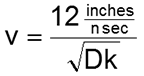
Signals propagate at roughly the speed of light in the transmitting material. The speed of light in material is 12 inches per nanosecond (the speed of light in air) divided by the square root of the material’s dielectric constant.
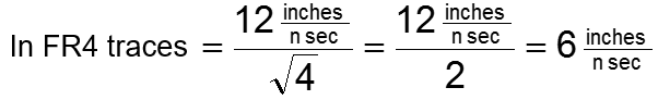
For an FR4 type printed circuit substrate material, the dielectric constant is 4, the square root of that is 2, and so 12 in divided by 2 is about 6 in per nanosecond. That is how fast a voltage signal can be expected to propagate through that material.
For an FR4 type printed circuit substrate material, the dielectric constant is 4, the square root of that is 2, and so 12 in divided by 2 is about 6 in per nanosecond. That is how fast a voltage signal can be expected to propagate through that material.
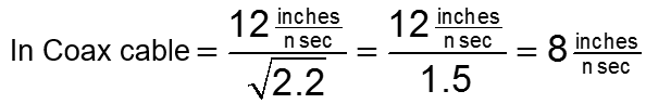
For the RG-174 coaxial cables used in our experiment, which have polyethylene dielectric material, the dielectric constant is 2.2, less than that of a circuit board, and so the propagation speed is a little faster, about 8 in per nanosecond.
For the RG-174 coaxial cables used in our experiment, which have polyethylene dielectric material, the dielectric constant is 2.2, less than that of a circuit board, and so the propagation speed is a little faster, about 8 in per nanosecond.
Travelling one way down a 1 ft coax cable takes about 1.5 ns and travelling 3 ft takes about 4.5 ns. When we measured a 228 ns rise time using a 3 ft cable, the time delay represented in that number was at most 5 ns. Where did the other 223 ns come from?
We’ll examine this and the dynamics of propagation more closely in our next post.
Copyright © 2020-2026 Teledyne LeCroy. All rights reserved. All original content, including text and photos, is the property of Teledyne LeCroy and cannot be reproduced without expressed written permission.

Accurate on-die power rail measurements depend on proper sense-line design, differential probing, and careful test setup at the package level.

Transmission line losses—driven by skin effect and dielectric properties—play a critical role in degrading high-speed signal integrity and eye performance.

Transmission line loss directly affects eye diagram quality, with around −12 dB at Nyquist marking the limit before signal integrity rapidly degrades without equalization.

This article explains how PDN design, probing method, and measurement location influence power rail noise—and why board-level measurements can be misleading.